Logistic regression
The problems we had with the perceptron were:
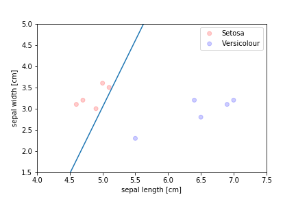
- only converged for linearly separable problems
- stopped places that did not look like they would generalise well
We need an algorithm that takes a more balanced approach:
- finds a "middle ground" decision boundary
- can make decisions even when the data is not separable
Logistic regression
- for binary classification for positive ($y=1$) vs negative ($y=0$) class
- for a probability $p$ to belong to the positive class, the odds ratio is given by $$ r=\frac{p}{1-p}$$
- if $r > 1$ we are more likely to be in the positive class
- if $r < 1$ we are more likely to be in the negative class
- to make it more symmetric we consider the log of $r$
- use a linear model for $z=log(r)$: $$ z= \omega_0 + \sum_j x_j w_j = w_0 + (x_1,...,x_D)\cdot (\omega_1,...,\omega_D) $$
If we set $x_0 = 1$ we can write this as
$$ z= \sum\limits_{j=0}^{n_f} x_j w_j = (x_0, x_1,...,x_D)\cdot (\omega_0, \omega_1,...,\omega_D) $$
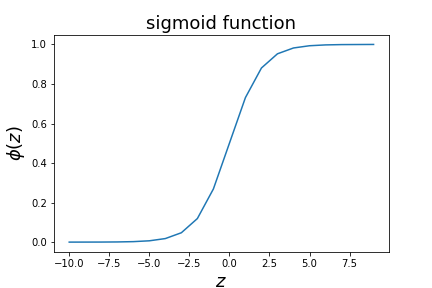
We can invert to obtain probability as a function of $z$ $$ p = \frac{1}{1+e^{-z}}\equiv \phi(z) $$
logistic regression optimisation
- the typicall loss function optimised for logistic regression is
$$J= - \sum_i y^{(i)} \log \left(\phi(z^{(i)}\right) +(1-y^{(i)})\log\left(1-\phi(z^{(i)}\right)$$
- only one of the log terms is activated per training data point
- if $y^{(i)}=0$ the loss has a term $\log(1-\phi(z^{(i)}))$
- the contribution to the loss is small if $z^{(i)}$ is negative (assigned correctly)
- the contribution to the loss is large if $z^{(i)}$ is positive (assigned incorrectly)
- if $y^{(i)}=1$ the loss has a term $\log(\phi(z^{(i)}))$
- the contribution to the loss is large if $z^{(i)}$ is negative (assigned incorrectly)
- the contribution to the loss is large if $z^{(i)}$ is positive (assigned correctly)
- if $y^{(i)}=0$ the loss has a term $\log(1-\phi(z^{(i)}))$
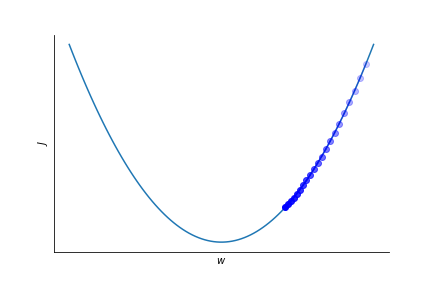
Gradient descent
To optimize the parameters $w$ in the logistic regression fit to the log of the probability we calculate the gradient of the loss function $J$ and go in opposite direction.
$$ w_{j} \rightarrow w_j -\eta \frac{\partial J}{\partial w_j} $$
$\eta$ is the learning rate, it sets the speed at which the parameters are adapted.
It has to be set empirically.
Finding a suitable $\eta$ is not always easy.
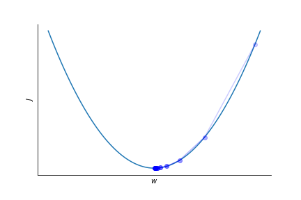
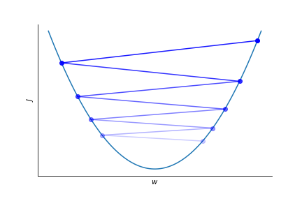
A too small learning rate leads to slow convergence.
Too large learning rate might spoil convergence altogether!
Gradient descent for logistic regression
$$ \frac{\partial \phi(z)}{\partial z} = - \frac{1}{(1 + e^{-z})^2} (-e^{-z}) = \phi(z) \frac{e^{-z}}{1 + e^{-z}} = \phi(z) (1-\phi(z)) $$
$$ \frac{\partial \phi}{\partial w_j} = \frac{\partial \phi(z)}{\partial z} \frac{\partial z}{\partial w_j} = \phi(z) (1-\phi(z)) x_j$$
$$ \begin{eqnarray} \frac{\partial J}{\partial w_j} &=& - \sum_i y_i \frac{1}{\phi(z_i)}\frac{\partial \phi}{\partial w_j} - (1-y_i)\frac{1}{1-\phi(z_i)}\frac{\partial \phi}{\partial w_j} \\ &=& - \sum_i y_i (1-\phi(z_i))x_j^{(i)} - (1-y_i)\phi(z_i)x_j^{(i)} \\ & = & - \sum_i (y_i - \phi(z_i)) x_j^{(i)} \end{eqnarray} $$
where $i$ runs over all data sample, $1\leq i \leq n_d$ and $j$ runs from 0 to $n_f$.
Loss minimization
Algorithms:
gradient descent method
Newton method: second order method Training:
use all the training data to compute gradient
use only part of the training data: Stochastic gradient descent
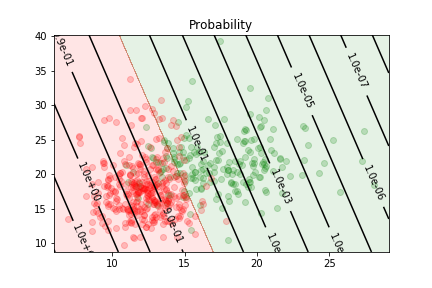
Logistic regression example
two features relevant to the discrimination of benign and malignent tumors:
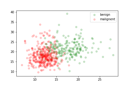
The data is not linearly separable.
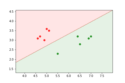
We can train a sigmoid model to discriminate between the two types of tumors. It will assign the output class according to the value of
$$z= w_0 + \sum_j w_j x_j = w_0 + (x_1,x_2) (\omega_1,\omega_2)^T $$
where $\omega_0$, $\omega_1$ and $\omega_2$ are chosen to minimize the loss.
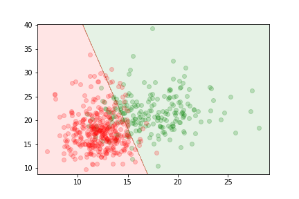
The delimitation is linear because the relationship between parameters and features in the model is linear.
The logistic regression gives us an estimate of the probability of an example to be in the first class
Normalising inputs
It is often important to normalise the features. We want the argument of the sigmoid function to be of order one.
- Too large or too small values push the problem into the "flat" parts of the function
- gradient is small
- convergence is slow
It is useful to normalise features such that their mean is 0 and their variance is 1.
Loss functions
Loss functions are used to quantify how well or bad a model can reproduce the values of the training set.
The appropriate loss function depends on the type of problems and the algorithm we use.
Let's denote with $\hat y$ the prediction of the model and $y$ the true value.
Gaussian noise
Let's assume that the relationship between the features $X$ and the label $Y$ is given by
$$ Y = f(X) +\epsilon$$where $f$ is the model whose parameters we want to fix and $\epsilon$ is some random noise with zero mean and variance $\sigma$.
The likelihood to measure $y$ for feature values $x$ is given by
$$L\sim \exp\left(-\frac{(y-f(x))^2}{2\sigma}\right) $$If we have a set of examples $x^{(i)}$ the likelihood becomes
$$ L\sim \prod_i \exp\left(-\frac{(y^{(i)}-f(x^{(i)}))^2}{2\sigma}\right) $$We now want to fix the parameters in $f$ such that we maximize the likelihood that our data was generated by the model.
It is more convenient to work with the log of the likelihood. Maximizing the likelihood is equivalent to minimising the negative log-likelihood.
$$ NLL = - \log(L) = \frac{1}{2\sigma} \sum_i \left(y^{(i)}-f(x^{(i)})\right)^2 $$So assuming gaussian noise for the difference between the model and the data leads to the least square rule.
We can use the square error loss
$$ J(f) = \sum_i \left(y^{(i)}-f(x^{(i)})\right)^2 $$To train our machine learning algorithm.
Two class model
If we have two classes, we call one the positive class ($c=1$) and the other the negative class ($c=0$). If the probability to belong to class 1
$$p(c=1) = p$$we also have
$$ p(c=0)=1-p $$The likelihood for a single measurement if the outcome is in the positive class is $p$ and if the outcome is in the negative class the likelihood is $1-p$. For a set of measurements with outcomes $y_i$ the likelihood is given by
$$ L = \prod\limits_{y_i=1} p \prod\limits_{y_i=0} (1-p) $$So the negative log-likelihood is:
$$ NLL = - \sum\limits_{y_i=1} \log(p) - \sum\limits_{y_i=0} \log(1-p) $$Given that $y=0$ or $y=1$ we can rewrite it as
$$ NLL = - \sum \left( y \log(p) + (1-y)\log(1-p) \right) $$So if we have a model for the probability $\hat y = p(X)$ we can maximize the likelihood of the training data by optimizing
$$ J= - \sum_i y_i \log \left(\hat y\right) +(1-y_i)\log\left(1 - \hat y\right) $$It is called the cross entropy.
Perceptron loss
One can formulate the perceptron algorithm in terms of a stochastic gradient descent with the loss given by
$$ J(w) = \sum h( y_i p(x_i,w))$$where $p(x_i,w)$ is the model prediction $\vec x\cdot \vec w + w_0$ and $h$ is the hinge function:
$$ h(x)=\left\{ \begin{array}{ccc} -x & \mbox{if} & x < 0 \\ 0 &\mbox{if}& x \ge 0 \end{array}\right. $$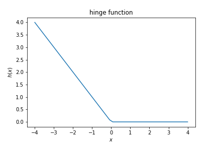
The loss for the SVM also uses the hinge function, but offset such that we penalise values up to 1:
$$ J(w) = \frac{1}{2}\vec w\cdot \vec w + C \sum h_1( y_i p(x_i,w)) $$where $p(x_i,w)$ is the model prediction $\vec x\cdot \vec w + w_0$ and $h_1$ is the shifted hinge function.
$$ h_1(x) = \max(0, 1- x).$$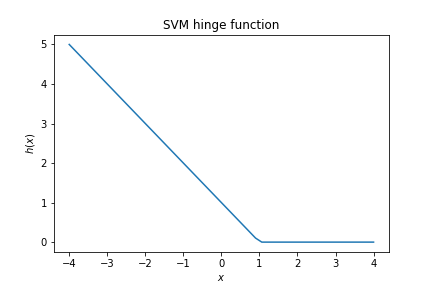
$C$ is a model parameter controlling the trade-off between the width of the margin and the amount of margin violation.