Summative assessment
- Released 2 pm 13th January 2025
- Collected 2 pm 14th January 2025
The same place as all the formative assignments, online for 24 hours and done remotely. It should not take 24 hours to complete! This is redundancy time incase of any problems with the server.
Summative assessment
The assigment will be an ML task to analyse a dataset using one or more techniques that we have covered in the lectures such as:
- Logistic regression (week 1)
- ROC (week 2)
- Non-linear models (week 2)
- Neural networks (week 3)
- PCA (week 4)
- kNN (week 4)
Summative assessment
Remember:
- The full notebook should run within 2 minutes, max 5 minutes but there is a buffer of up to 10 minutes which is plenty!
- Make sure to 'Restart & Run All' before you submit to check that your code runs in good time and appears how you want it to.
- No collusion (this is an individual assignment).
- Don't use generative AI.
- All code will be reviewed.
The curse of dimensionality
One would think that the more features one has to describe samples in a dataset the better one would be able to perform a classification task. Unfortunately with the increase of the number of features comes the difficulty of fitting a multi-dimensional model.
This is generally referred to as the curse of dimensionality and we will see a few surprising effects that explain why more features can make life difficult.
How many points are in the center of the cube?
We can ask the question "In the hypercube $-1\leq x_i\leq 1$, how many points are no further apart to the center than 1?"
This is equivalent to asking what is the ratio of the unit "ball" to the volume of the smallest "cube" enclosing it.
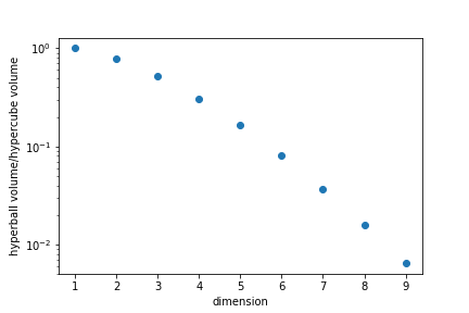
In high dimensions most points are in "corners" rather than in the "centre".
Average distance between two random points
Looking at the unit cube, we can calculate the average distance between any two points.
$$ d=\sqrt{\sum_i x_i^2} $$
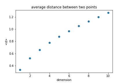
The average distance increases with the dimension.
We can also plot the distribution of distances:
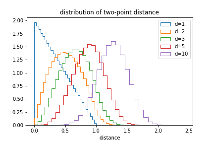
The likelihood of small distances drops as the dimension increases.
Proximity to edges
One interesting question to ask is how close to the edges points are. To quantify it we will calculate what is the thickness $t$ of the outer layer of the unit cube that contain half the points if the points are randomly distributed.
The volume inside is given by
$$ V_i = (1-2t)^d \qquad V_i=\frac12 \Rightarrow t = \frac{1-2^{-1/d}}{2}$$
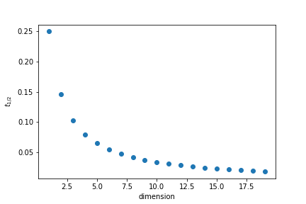
In 35 dimensions half of the points are in a outer layer 0.01 thin.
Principal component analysis
If we have many features, odds are that many are correlated. If there are strong relationships between features, we might not need all of them.
With principal component analysis we want to extract the most relevant/independant combination of features.
It is important to realise that PCA only looks at the features without looking at the labels, it is an example of unsupervised learning.
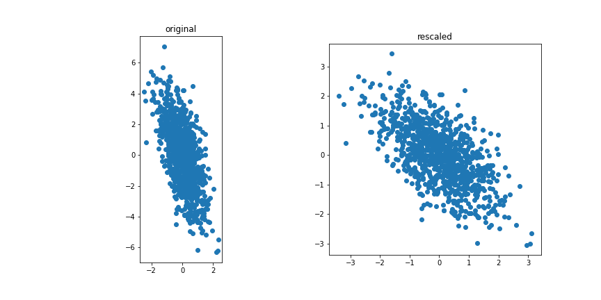
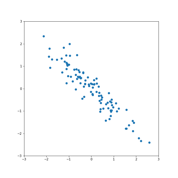
Correlated vs uncorrelated
Correlated features
Uncorrelated features:
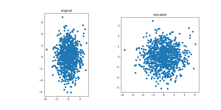
The idea for PCA is to project the (standardised) data on a subspace with fewer dimensions.
Standardization
Standarization involves transforming data so that each feature has a mean of 0 and a standard deviation of 1.
PCA is sensitive to the scale of the variables. Features with larger scales can dominate the principal components, skewing the results.
Illustrative Example:
- Consider a dataset with two features: height (in centimeters) and weight (in kilograms).
- Without standardization, height might dominate because its numerical values are larger.
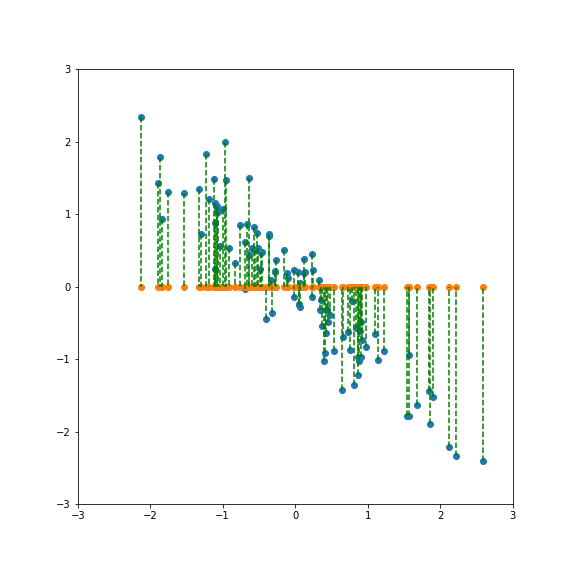
If we project onto the first component we get variance 1:
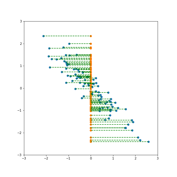
If we project onto the second component we also get variance 1:
But projecting onto a different direction gives a different variance, here larger than 1:
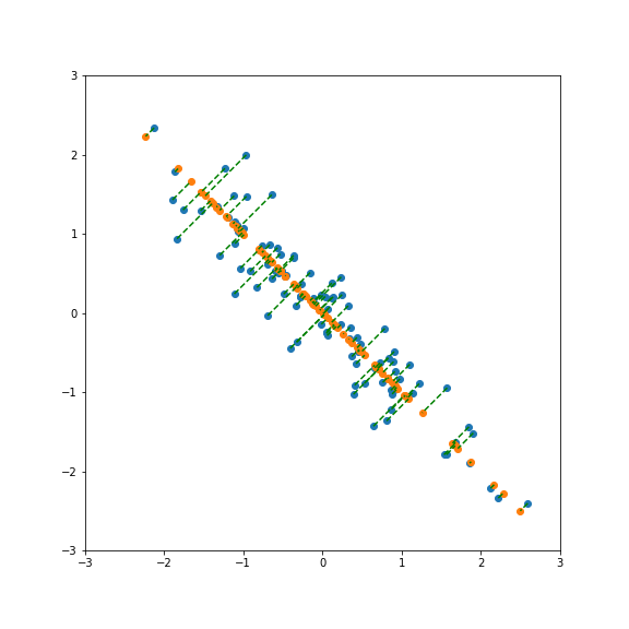
And here smaller than one:
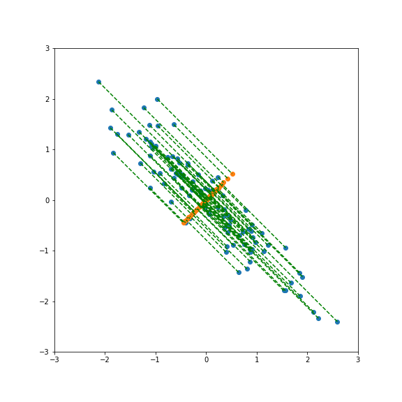
Performing PCA gives a new basis in feature space that include the direction of largest and smallest variance.
There is no guarantee that the most relevant features for a given classification tasks are going to have the largest variance.
If there is a strong linear relationship between features it will correspond to a component with a small variance, so dropping it will not lead to a large loss of variance but will reduce the dimensionality of the model.
Finding the principal components
The first step is to normalise and center the features.
$$ x_i \rightarrow a x_i +b $$such that
$$ \langle x_i\rangle = 0 \;,\qquad \langle x_i^2\rangle = 1$$The covariance matrix of the data is then given by
$$ \sigma = X^T X $$If $X$ is the $n_d\times n_f$ data matrix of the $n_d$ training samples with $n_f$ features. The covariance matrix is a $n_f\times n_f$ matrix.
Explained variance
When we only consider the $k$ principal axis of a dataset we will lose some of the variance of the dataset.
Assuming the eigenvalues are ordered in size we have
$$\sigma_k\equiv {\rm{Tr}}(X_k^T X_k) = \sum\limits_{j=1}^k \epsilon_j^2$$$\sigma_k$ is the variance our reduced dataset retained from the original, it is often referred as the explained variance.
Example: 8x8 digits pictures
We consider a dataset of handwritten digits, compressed to an 8x8 image:
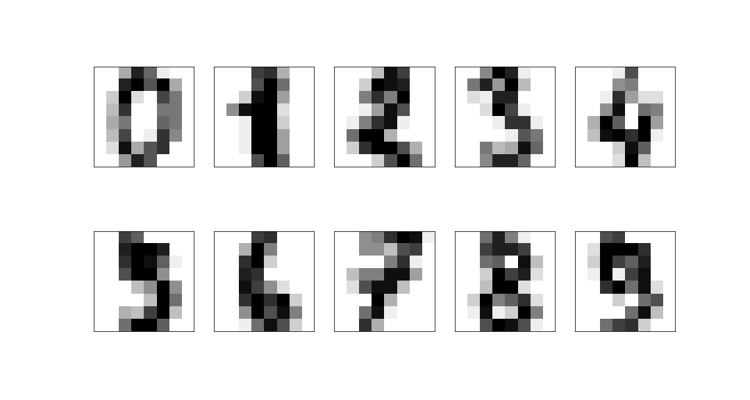
These have a 64-dimensional space but this is clearly far larger than the true dimension of the space:
- only a very limited subset of 8x8 pictures represent digits
- the corners are largely irrelevant hardly ever used
- digits are lines, so there is a large correlation between neighbouring pixels.
PCA should help us limit our features to things that are likely to be relevant.
Performing PCA we can see how many eigenvectors are needed to reproduce a given fraction of the dataset variance via a cumulative scree plot:

We can keep 50% of the dataset variance with less than 10 features.
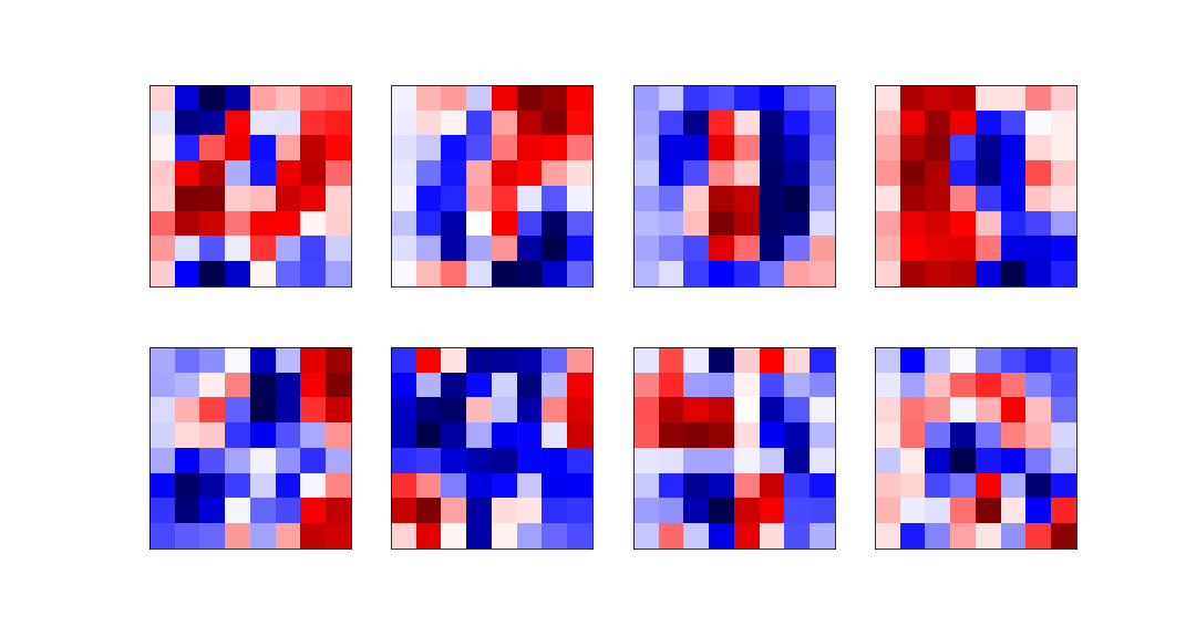
The eight most relevant eigenvectors are:
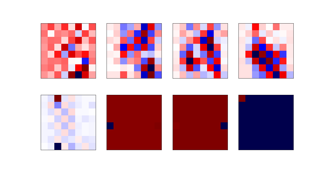
The least relevant eigenvectors are:
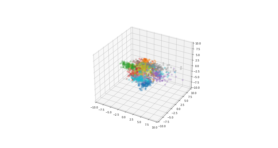
Data visualisation
If we reduce the data to be 2-dimensional or 3-dimensional we can get a visualisation of the data.
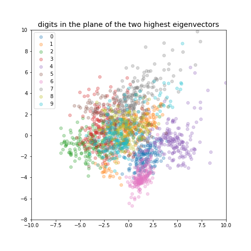
digits in the plane of the two highest eigenvectors
k-Neighbours
KNN
The parameter $k$ can be used to control overfitting.
- KNN is non-parametric (it makes no assumptions about the data's underlying distribution)
- KNN is lazy (it defers computation until the prediction phase).
- There's essentially no explicit training. KNN simply stores the training data.
- Basic procedure is compute distances, identify the 'k' closest data points, vote/average the class.
K-Nearest Neighbors (KNN)
The $k$-nearest neighbors method is an instance-based learning algorithm.
- It memorizes the training set.
- For a new data point, it finds the $k$ closest samples from the training set.
- Returns:
- Regression: The average of the target values of these $k$ neighbors.
- Classification: The class most common among the $k$ neighbors.
Intuition Behind KNN
Key Idea: Similar data points are likely to have similar target values.
- KNN uses the idea of proximity to predict the target variable.
- No explicit model is trained; all computations are deferred until prediction.
Advantages:
- Simple to understand and implement.
- Non-parametric: Makes no assumptions about data distribution.
Disadvantages:
- Computationally intensive with large datasets.
- Performance depends on the choice of $k$ and the distance metric.
Importance of Distance Metrics
Common Distance Metrics:
- Euclidean Distance: Straight-line distance between two points.
- Manhattan Distance: Sum of absolute differences along each dimension.
- Minkowski Distance: Generalization that includes both Euclidean and Manhattan.
Impact on KNN:
- The choice of distance metric affects which neighbors are considered "closest."
- Different metrics may be more appropriate depending on the data.
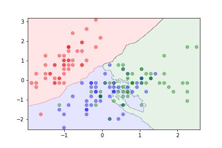
Regularisation
The parameter $k$ can be used to control overfitting.
- With $k=1$ the algorithm is likely to overfit.
- Large values of $k$ can lead to underfitting.
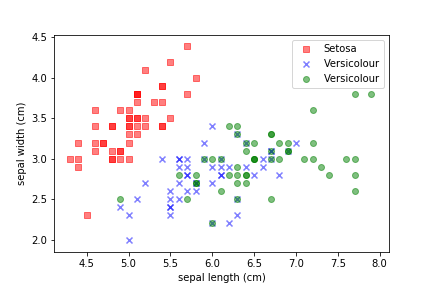
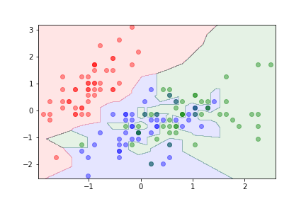
Example
We can use the iris dataset:
k=1
k =3
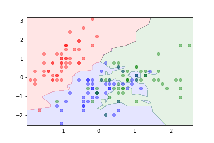
k=10
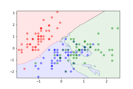
k=20
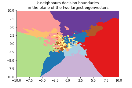
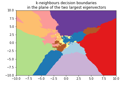
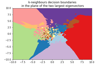
Digits example
We can use the 8x8 digits picture example after applying PCA to reduce it to 2 dimensions:
k=1
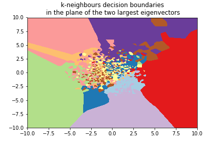
k=3
k=5