Neural Networks

An Introduction to Neural Networks and Deep Learning

Introduction to Neural Networks

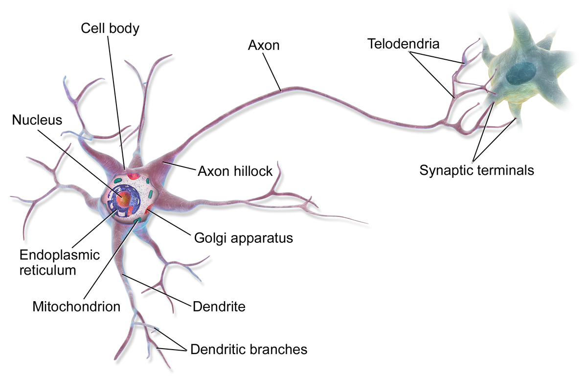
Neural networks are computational models inspired by the human brain's interconnected network of neurons.

Consist of layers of interconnected nodes called neurons .
Each neuron processes input and passes the output to the next layer.
Capable of learning complex patterns from data.
Used in various domains like computer vision, natural language processing, and more.

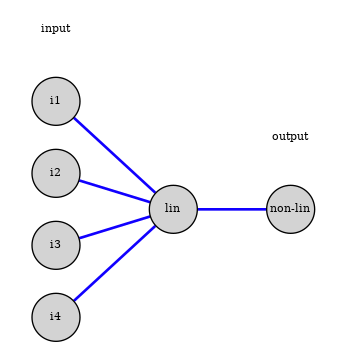
Artificial Neuron Model

A modern neuron in a neural network performs two main operations:

Linear Combination: Computes a weighted sum of inputs.
Non-linear Activation: Applies an activation function to introduce non-linearity.

Mathematically:

$$ z = w_0 + \sum_{i=1}^{n} w_i x_i $$

$$ \text{output} = \phi(z) $$

where $\phi(z)$ is the activation function.

Biological vs. Artificial Neurons

Biological Neurons	Artificial Neurons
Receive input signals via dendrites. Process signals in the cell body. Transmit signals via axons.	Receive inputs and weights. Compute a weighted sum. Apply an activation function.

The Perceptron Model

The perceptron is the simplest type of artificial neural network:

Introduced by Frank Rosenblatt in 1958.
Models a single neuron.
Performs binary classification.
Serves as the building block for more complex networks.

Mathematical Formulation of the Perceptron

Mathematically, the perceptron computes:

$$ z = w_0 + \vec{w} \cdot \vec{x} $$

$$ \text{output} = \phi(z) $$

where:

$\vec{x}$ = input vector.
$\vec{w}$ = weight vector.
$w_0$ = bias term.
$\phi(z)$ = activation function (e.g., step function).

The perceptron learning rule updates weights based on the error:

$$ w_j \leftarrow w_j + \eta (y - \hat{y}) x_j $$

where:

$\eta$ = learning rate.
$y$ = true label.
$\hat{y}$ = predicted label.

Limitations of the Perceptron

The perceptron has significant limitations:

Can only solve linearly separable problems.
Cannot model complex, non-linear decision boundaries (e.g., XOR problem).
Limited representational capacity.
Led to the development of multi-layer networks to overcome these limitations.

Multi-Layer Networks

Also known as Multi-Layer Perceptrons (MLPs).

Consist of an input layer, one or more hidden layers, and an output layer.
Hidden layers enable the network to learn complex, non-linear patterns.
Universal approximation theorem: MLPs can approximate any continuous function.

Multi-Layer Networks

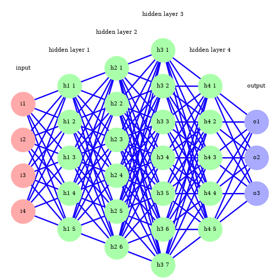
Deep Learning

Networks with a large number of layers are referred to as deep learning .

Advantages:

Can learn hierarchical representations.
Effective in processing high-dimensional data like images, speech, and text.

Challenges:

Require large amounts of data.
Computationally intensive training.
Potential for overfitting.

Advances in hardware (GPUs, TPUs) and algorithms (e.g., optimization techniques) have made deep learning feasible.

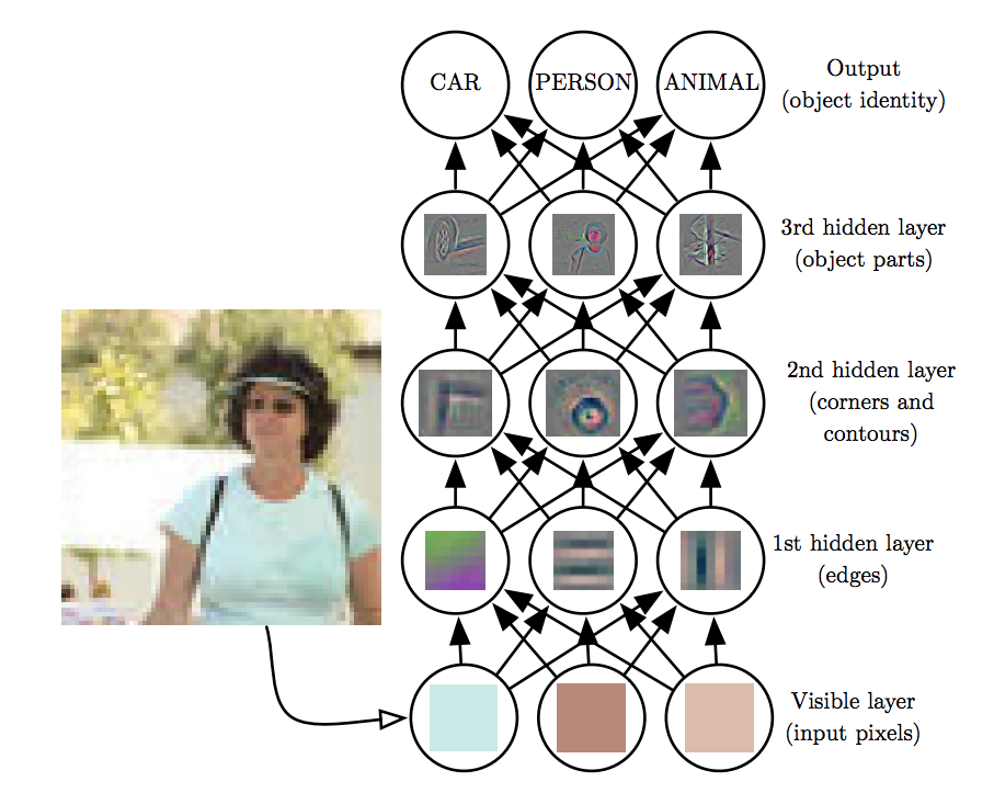
Deep Learning and Hierarchical Feature Learning

Deep learning leverages multiple layers to learn hierarchical representations:

Lower Layers: Capture simple features like edges or textures.
Middle Layers: Combine simple features to form more complex patterns.
Higher Layers: Abstract high-level concepts relevant to the task.

This hierarchy enables neural networks to automatically learn features from raw data.

Deep Learning and Hierarchical Feature Learning

Example: Circle Dataset

Using a neural network to classify points in a circular pattern:

Data is not linearly separable.
Single-layer networks fail to classify correctly.
Multi-layer networks with hidden units can capture the circular pattern.

Example: Iris Dataset

Classifying iris flowers into three species using a neural network:

Features: sepal length, sepal width, petal length, petal width.
Three classes: Setosa, Versicolor, Virginica.
Multi-class classification using softmax output layer.

Training Neural Networks

Training involves adjusting weights to minimize a loss function:

Initialize weights randomly or using specific initialization methods.
Perform a forward pass to compute the output.
Calculate the loss using a suitable loss function.
Compute gradients via backpropagation.
Update weights using an optimization algorithm.
Repeat the process for multiple epochs.

Key concepts:

Epoch: One complete pass through the training dataset.
Batch Size: Number of samples processed before updating weights.
Learning Rate: Controls the step size during weight updates.

Training Neural Networks

Training involves adjusting weights to minimize a loss function:

Initialize weights randomly or using specific initialization methods.
Perform a forward pass to compute the output.
Calculate the loss using a suitable loss function.
Compute gradients via backpropagation.
Update weights using an optimization algorithm.
Repeat the process for multiple epochs.

Weight Initialization Techniques

Proper weight initialization can help in faster convergence:

Zero Initialization: Not recommended as it causes symmetry.
Random Initialization: Small random values from a normal or uniform distribution.
Xavier Initialization: Scales weights based on the number of input and output neurons.
He Initialization: Similar to Xavier but designed for ReLU activation functions.

Avoiding vanishing or exploding gradients through appropriate initialization.

Training Neural Networks

Training involves adjusting weights to minimize a loss function:

Initialize weights randomly or using specific initialization methods.
a forward pass to compute the output.
Calculate the loss using a suitable loss function.
Compute gradients via backpropagation.
Update weights using an optimization algorithm.
Repeat the process for multiple epochs.

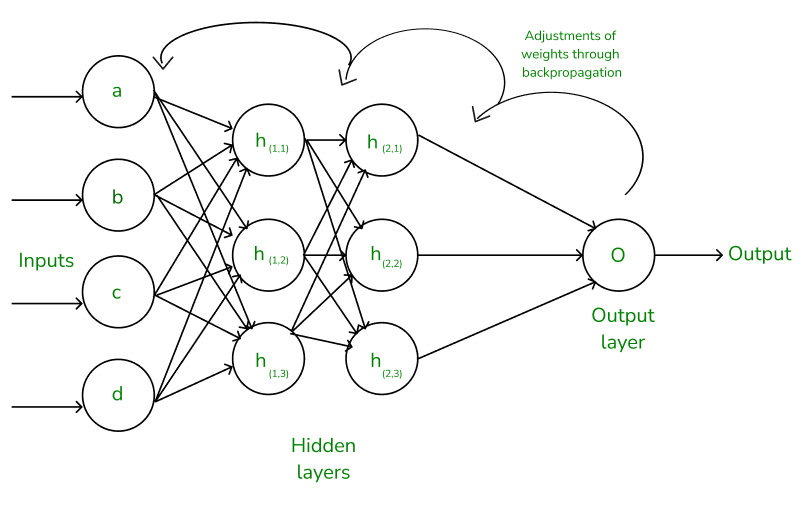
Feedforward Process

The feedforward process involves propagating inputs through the network to generate an output.

Input data is presented to the input layer.
Each neuron computes a weighted sum of its inputs and applies an activation function.
The outputs of one layer become the inputs to the next layer.
The final output layer produces the network's prediction.

This process is used during both training and inference phases.

Feedforward Process

Activation Functions

Activation functions introduce non-linearity into the neural network, allowing it to learn complex patterns.

Common activation functions include:

Step Function
Sigmoid Function
Tanh Function
ReLU (Rectified Linear Unit)
Leaky ReLU
ELU (Exponential Linear Unit)
Softmax Function

Selection of activation functions can significantly impact the network's performance.

Activation Functions

Step Function
- Formula:
  $$\phi(x) = \begin{cases} 1 & \text{if } x \geq 0 \\ 0 & \text{if } x < 0 \end{cases}$$
- Characteristics:
  - Binary output (0 or 1).
  - Non-differentiable at $ x = 0 $.
  - Historically used in perceptrons but less common in modern networks.

Activation Functions

Sigmoid Function

Formula:
$$\phi(x) = \frac{1}{1 + e^{-x}}$$
Characteristics:
- Output ranges between 0 and 1.
- Smooth and differentiable.
- Can cause vanishing gradient problems in deep networks.

Activation Functions

Tanh Function
Formula:
$$\phi(x) = \tanh(x) = \frac{e^{x} - e^{-x}}{e^{x} + e^{-x}}$$
Characteristics:
- Output ranges between -1 and 1.
- Zero-centered, which can be advantageous.
- Also susceptible to vanishing gradients.

Activation Functions

ReLU (Rectified Linear Unit)

Formula:
$$\phi(x) = \max(0, x)$$
Characteristics:
- Outputs zero for negative inputs and linear for positive inputs.
- Simple and computationally efficient.
- Helps mitigate vanishing gradient problems.
- Can suffer from "dying ReLUs" where neurons stop activating.

Advanced Activation Functions

Leaky ReLU
Formula:
$$\phi(x) = \begin{cases} x & \text{if } x \geq 0 \\ \alpha x & \text{if } x < 0 \end{cases}$$
Typically, $ \alpha $ is a small constant like 0.01.
Characteristics:
- Allows a small, non-zero gradient when $ x < 0 $.
- Addresses the "dying ReLU" problem.

Advanced Activation Functions

Softmax Function

Formula:
$$\phi(x_i) = \frac{e^{x_i}}{\sum_{j} e^{x_j}}$$
Characteristics:
- Converts logits into probabilities that sum to 1.
- Commonly used in the output layer for multi-class classification.

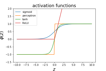
Non-linear activation functions¶

There are different decision functions that can be used.

the perceptron used a step function
logistic regression uses the sigmoid function
one can also use $\phi(z)=tanh(z)$ as a decision function
various variations on the hinge function (ReLU)

Training Neural Networks

Training involves adjusting weights to minimize a loss function:

Initialize weights randomly or using specific initialization methods.
Perform a forward pass to compute the output.
Calculate the loss using a suitable loss function.
Compute gradients via backpropagation.
Update weights using an optimization algorithm.
Repeat the process for multiple epochs.

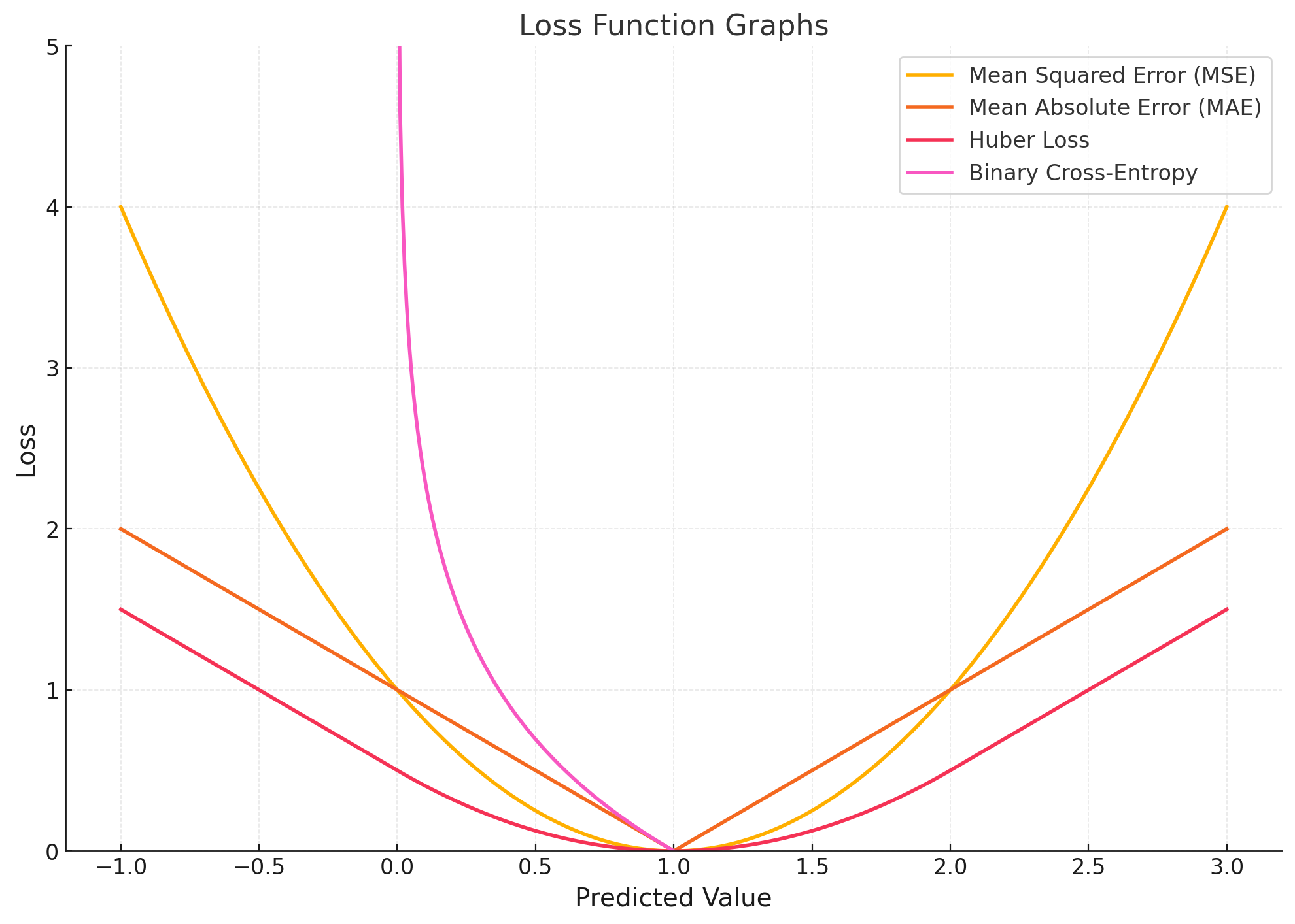
Loss Functions

Loss functions quantify the difference between the predicted output of the network and the true output. They are crucial for training neural networks using backpropagation.

Common loss functions include:

Mean Squared Error (MSE)
Mean Absolute Error (MAE)
Binary Cross-Entropy Loss (Log Loss)
Categorical Cross-Entropy Loss
Hinge Loss
Kullback-Leibler Divergence Loss (KL Divergence)

Loss Functions

Mean Squared Error (MSE)
- Formula:
  $$L_{\text{MSE}} = \frac{1}{n} \sum_{i=1}^{n} (y_i - \hat{y}_i)^2$$
- Explanation:
  - $ y_i $: True value.
  - $ \hat{y}_i $: Predicted value.
  - Measures the average squared difference between predictions and actual values.
- Usage:
  - Commonly used in regression problems.
  - Penalizes larger errors more than smaller ones.

Loss Functions

Mean Absolute Error (MAE)

Formula:
$$L_{\text{MAE}} = \frac{1}{n} \sum_{i=1}^{n} |y_i - \hat{y}_i|$$
Explanation:
- Measures the average absolute difference between predictions and actual values.
Usage:
- Used in regression problems where outliers are less significant.
- Less sensitive to outliers compared to MSE.

Loss Functions

Binary Cross-Entropy Loss (Log Loss)

Formula:
$$L_{\text{Binary}} = -\frac{1}{n} \sum_{i=1}^{n} [ y_i \log(\hat{y}_i) + (1 - y_i) \log(1 - \hat{y}_i) ]$$
Explanation:
- Used for binary classification tasks.
- Penalizes the divergence between predicted probabilities and actual labels.
Usage:
- Applicable when outputs are probabilities (using sigmoid activation in the output layer).

Loss Functions

Categorical Cross-Entropy Loss

Formula:
$$L_{\text{Categorical}} = -\sum_{i=1}^{n} \sum_{k=1}^{K} y_{i,k} \log(\hat{y}_{i,k})$$
Explanation:
- $ y_{i,k} $: Binary indicator (0 or 1) if class label $ k $ is the correct classification for sample $ i $.
- $ \hat{y}_{i,k} $: Predicted probability that sample $ i $ is of class $ k $.
- Used for multi-class classification tasks.
Usage:
- Often used with softmax activation in the output layer.

Loss Functions

Hinge Loss

Formula:
$$L_{\text{Hinge}} = \frac{1}{n} \sum_{i=1}^{n} \max(0, 1 - y_i \hat{y}_i)$$
Explanation:
- Used primarily for "maximum-margin" classification, especially with support vector machines.
- $ y_i $ should be -1 or 1, representing class labels.
Usage:
- Can be used in neural networks for binary classification.

Loss Functions

Kullback-Leibler Divergence Loss (KL Divergence)

Formula:
$$L_{\text{KL}} = \sum_{i=1}^{n} y_i \log\left( \frac{y_i}{\hat{y}_i} \right)$$
Explanation:
- Measures how one probability distribution diverges from a second, expected probability distribution.
Usage:
- Used in applications like variational autoencoders.

Loss Functions

Role in Backpropagation:

The loss function calculates the error between the network's predictions and the true values.
The computed loss is then used to calculate gradients during backpropagation.
The gradients are propagated backward through the network to update the weights.

Understanding and selecting the appropriate loss function is critical for effective training of neural networks.

Training Neural Networks

Training involves adjusting weights to minimize a loss function:

Initialize weights randomly or using specific initialization methods.
Perform a forward pass to compute the output.
Calculate the loss using a suitable loss function.
Compute gradients via backpropagation.
Update weights using an optimization algorithm.
Repeat the process for multiple epochs.

Backpropagation

Backpropagation is the algorithm used to train neural networks:

Computes the gradient of the loss function with respect to each weight by the chain rule.
Updates weights in the opposite direction of the gradient.
Repeats the process for multiple iterations (epochs).

Training Neural Networks

Training involves adjusting weights to minimize a loss function:

Initialize weights randomly or using specific initialization methods.
Perform a forward pass to compute the output.
Calculate the loss using a suitable loss function.
Compute gradients via backpropagation.
Update weights using an optimization algorithm.
Repeat the process for multiple epochs.

Gradient Descent

Gradient descent is the optimization algorithm used to minimize the loss function.

Update rule:

$$ w_{ij} = w_{ij} - \eta \frac{\partial J}{\partial w_{ij}} $$

where:

$\eta$ = learning rate.
$\frac{\partial J}{\partial w_{ij}}$ = gradient of the loss with respect to weight $w_{ij}$.

Variants:

Batch Gradient Descent
Stochastic Gradient Descent (SGD)
Mini-Batch Gradient Descent

Optimization Algorithms

Various optimization algorithms improve training efficiency and convergence:

Stochastic Gradient Descent (SGD): Updates weights using individual samples.
Momentum: Accelerates SGD by considering past gradients.
Adagrad: Adapts learning rate based on past gradients.

Choice of optimizer can significantly affect training performance.

Optimization Algorithms

Various optimization algorithms improve training efficiency and convergence:

Stochastic Gradient Descent (SGD)
- Update Rule:
  $$w_{t+1} = w_t - \eta \nabla L(w_t; x_i, y_i)$$
- Explanation:
  - Updates weights using individual samples $ (x_i, y_i) $.
  - $ \eta $ is the learning rate.
  - $ \nabla L(w_t; x_i, y_i) $ is the gradient of the loss function at time $ t $.
- Characteristics:
  - Introduces noise due to sampling, which can help escape local minima.
  - Can be slow to converge near minima.

Optimization Algorithms

Momentum

Update Rule:
$$\begin{align*} v_{t} & = \gamma v_{t-1} + \eta \nabla L(w_t) \\ w_{t+1} & = w_t - v_{t} \end{align*}$$
Explanation:
- $ v_t $ is the velocity (accumulated gradient).
- $ \gamma $ is the momentum coefficient (typically between 0 and 1).
- Accelerates SGD by smoothing gradients over time.
Characteristics:
- Helps navigate ravines in the loss surface.
- Can overshoot minima if $ \gamma $ is too high.

Optimization Algorithms

Adagrad

Update Rule:
$$\begin{align*} G_t & = G_{t-1} + \nabla L(w_t)^2 \\ w_{t+1} & = w_t - \frac{\eta}{\sqrt{G_t + \epsilon}} \nabla L(w_t) \end{align*}$$
Explanation:
- $ G_t $ is the sum of the squares of past gradients (element-wise).
- $ \epsilon $ is a small constant to prevent division by zero (e.g., $ 10^{-8} $).
- Adapts the learning rate for each parameter individually.
Characteristics:
- Good for sparse data.
- Learning rate diminishes over time, which can halt training prematurely.

Training Neural Networks

Training involves adjusting weights to minimize a loss function:

Initialize weights randomly or using specific initialization methods.
Perform a forward pass to compute the output.
Calculate the loss using a suitable loss function.
Compute gradients via backpropagation.
Update weights using an optimization algorithm.
Repeat the process for multiple epochs.

Challenges in Training Deep Networks

Deep networks introduce specific challenges:

Vanishing Gradients: Gradients become very small, slowing down learning.
Exploding Gradients: Gradients grow exponentially, causing instability.
Overfitting: Model performs well on training data but poorly on unseen data.
Computational Complexity: Increased number of parameters requires more computational resources.

Strategies to mitigate these issues include activation function choices, gradient clipping, and regularization.

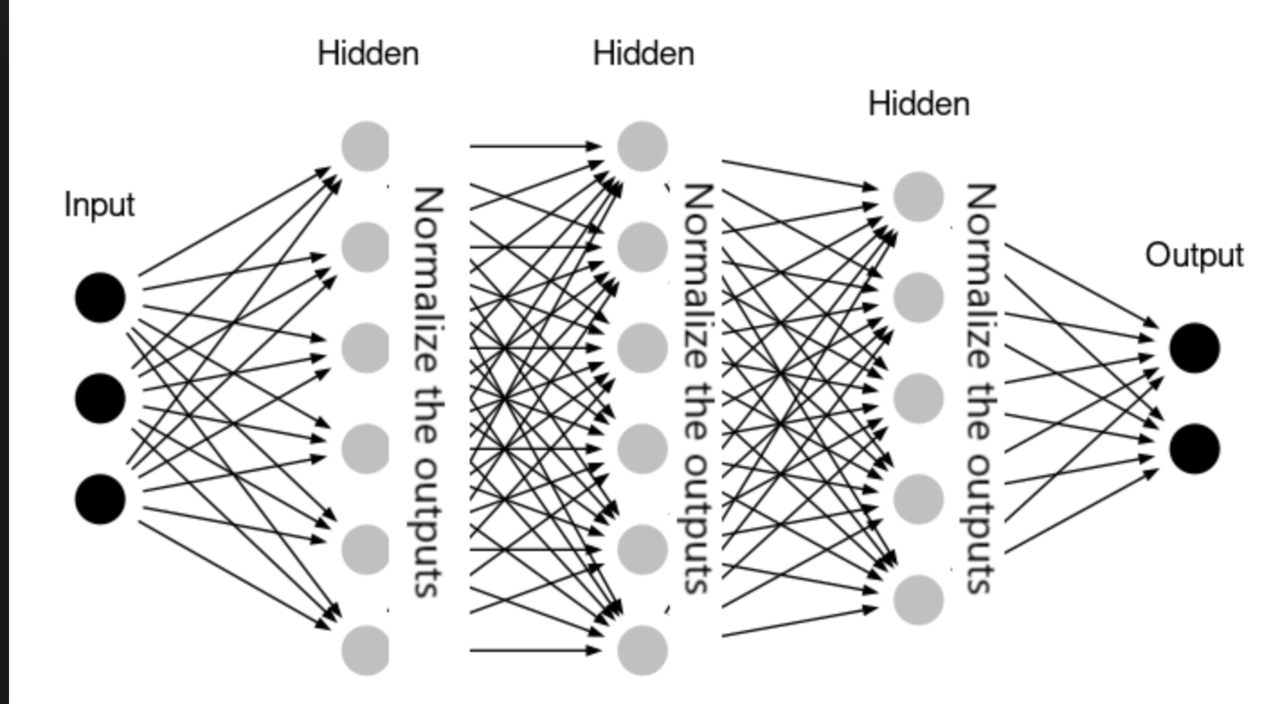
Batch Normalization

Batch normalization is a technique to improve training speed and stability:

Normalizes the input of each layer to have zero mean and unit variance.
Reduces internal covariate shift.
Allows for higher learning rates.
Acts as a form of regularization.

Introduced by Sergey Ioffe and Christian Szegedy in 2015.

Batch Normalization

Regularization Techniques

To prevent overfitting, we use regularization methods:

L1 and L2 Regularization: Add penalty terms to the loss function.
Dropout: Randomly drop units during training to prevent co-adaptation.
Early Stopping: Stop training when validation loss starts to increase.
Data Augmentation: Increase the size of the training data by transformations.
Ensemble Methods: Combine multiple models to improve generalization.

Regularization helps in building models that generalize well to new data.

Practical Considerations

Important aspects to consider when working with neural networks:

Hyperparameter Tuning: Selecting learning rates, batch sizes, number of layers, etc.
Data Preprocessing: Normalization, scaling, and handling missing data.
Hardware Acceleration: Utilizing GPUs and TPUs for faster computation.
Frameworks and Libraries: TensorFlow, PyTorch, Keras, etc.
Model Interpretability: Understanding and explaining model decisions.

These factors can significantly impact the performance and usability of neural network models.

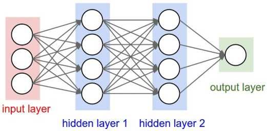
Network Architectures

Neural networks are constructed by connecting artificial neurons in various configurations.

Types of network architectures:

Feedforward Neural Networks: Information moves only in one direction, from input to output.
Convolutional Neural Networks (CNNs): Specialized for processing grid-like data such as images.
Recurrent Neural Networks (RNNs): Designed for sequential data, with loops to allow information to persist.
Autoencoders: Used for unsupervised learning of efficient codings.
Generative Adversarial Networks (GANs): Consist of generator and discriminator networks for data generation.
Transformer Networks: Utilize self-attention mechanisms, prominent in NLP tasks.

Each architecture is tailored for specific types of data and tasks.

Advanced Topics in Deep Learning

Exploring cutting-edge developments in deep learning:

Attention Mechanisms: Allow models to focus on specific parts of the input.
Transfer Learning: Leveraging pre-trained models for new tasks.
Generative Models: GANs and Variational Autoencoders (VAEs).
Self-Supervised Learning: Learning representations from unlabeled data.
Reinforcement Learning: Training agents to make decisions through rewards.

These topics represent the forefront of research and applications in deep learning.

Examples and Applications

Neural networks are used in various fields:

Computer Vision: Image classification, object detection, image segmentation.
Natural Language Processing: Language translation, sentiment analysis, question answering.
Speech Recognition: Voice assistants, transcription services, speech synthesis.
Healthcare: Disease prediction, medical image analysis, personalized medicine.
Finance: Fraud detection, stock price prediction, algorithmic trading.
Autonomous Vehicles: Perception, decision-making, and control systems.

These applications showcase the versatility and impact of neural networks.

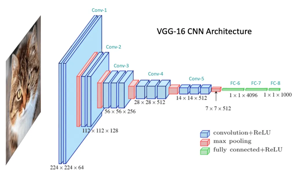
Case Study: Convolutional Neural Networks

Understanding CNNs through image classification tasks:

Convolution Layers: Extract spatial features using filters.
Pooling Layers: Reduce spatial dimensions and control overfitting.
Fully Connected Layers: Perform classification based on extracted features.
Applications: Used in models like AlexNet, VGGNet, ResNet.

Case Study: Convolutional Neural Networks

Conclusion

Neural networks are powerful tools for modeling complex patterns in data.

Key takeaways:

They consist of interconnected neurons with activation functions.
Can model non-linear relationships using hidden layers.
Training involves feedforward and backpropagation processes.
Regularization is essential to prevent overfitting.
They have widespread applications across various domains.
Continuous advancements are expanding their capabilities.

Understanding the fundamentals allows for further exploration into advanced topics.

Thank you for your attention!

Variance Bias Trade-off¶

What is Bias and Variance?

Bias: The error introduced by approximating a real-world problem, which may be complex, by a much simpler model.

High bias can cause an algorithm to miss relevant relations between features and target outputs (underfitting).

Variance: The error introduced by the model's sensitivity to fluctuations in the training set.

High variance can cause overfitting, where the model captures noise in the data.

Let's suppose the relationship between $X$ and $Y$ is described by

$$ Y = \sum_i w_i^\star x^i + \epsilon$$

where $w_i^\star$ are the true parameters and $\epsilon$ is some noise.

We will try to model this with

$$ y = p(x) = \sum_i w_i x^i$$

where now the $w_i$ will be fitted to data.

We define

$$ \bar w_i = \langle w_i\rangle $$

as the expectation value of the parameter $w_i$ when fitted to multiple independent samples drawn from the true distribution.

We want to calculate the expected deviation of the fitted coefficients form the true coefficient:

$$ \langle (w_i-w_i^\star)^2\rangle$$

$$ \begin{eqnarray} \langle (w_i-w_i^\star)^2\rangle & = & \langle (w_i-\bar w_i +\bar w_i -w_i^\star)^2\rangle \\ &=& \langle (w_i-\bar w_i)^2\rangle + \langle (\bar w_i-w_i^\star)^2\rangle +2 \langle (w_i-\bar w_i)(\bar w_i -w_i^\star)\rangle \end{eqnarray}$$

The third term vanishes: $$ \langle (w_i-\bar w_i)(\bar w_i -w_i^\star)\rangle = \langle (w_i-\bar w_i)\rangle (\bar w_i -w_i^\star) =0 $$

So we have

$$ \langle (w_i-w_i^\star)^2\rangle = \langle (w_i-\bar w_i)^2\rangle + \langle (\bar w_i-w_i^\star)^2\rangle$$

The first term is the variance term and the second is the bias.

Example¶

To illustrate the variance-bias tradeoff we will be using different models to describe data with true relationship between the input $x$ and the outcome

$$Y(x) = 1+\frac15 x^2 + \epsilon \qquad \mbox{for}\qquad 0\leq x\leq 1\;, \quad 0 \; \mbox{otherwise}$$

Where $\epsilon$ is a gaussian noise. We will use the two models

$$ m_1(x) = a +bx$$

and

$$m_2(x)= a+bx +cx^2 +dx^3.$$

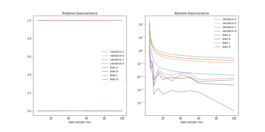
Using $m_1$, a model with too few parameters we get

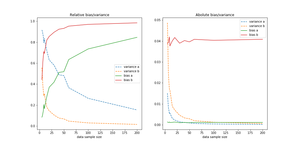
For low dataset size we see the the variance dominates but as the number of training samples grows the bias dominates. Since the model is not capable of describing the truth the error is not diminishing even though the variance part of the error drops proportional to $1/\sqrt{N}$

For the second model where we have enough freedom to exactly describe the truth we get: